
Recommendation
 based on reviews by Guillaume Achaz, Jere Koskela, William Shoemaker and Simon Boitard
Many organisms across the Tree of life have the ability to produce seeds, eggs, cysts, or spores, that can remain dormant for several generations before hatching. This widespread adaptive trait in bacteria, fungi, plants and animals, has a significant impact on the ecology, population dynamics and population genetics of species that express it (Evans and Dennehy 2005).
In population genetics, and despite the recognition of its evolutionary importance in many empirical studies, few theoretical models have been developed to characterize the evolutionary consequences of this trait on the level and distribution of neutral genetic diversity (see, e.g., Kaj et al. 2001; Vitalis et al. 2004), and also on the dynamics of selected alleles (see, e.g., Živković and Tellier 2018). However, due to the complexity of the interactions between evolutionary forces in the presence of dormancy, the fate of selected mutations in their genomic environment is not yet fully understood, even from the most recently developed models.
In a comprehensive article, Korfmann et al. (2023) aim to fill this gap by investigating the effect of germ banking on the probability of (and time to) fixation of beneficial mutations, as well as on the shape of the selective sweep in their vicinity. To this end, Korfmann et al. (2023) developed and released their own forward-in-time simulator of genome-wide data, including neutral and selected polymorphisms, that makes use of Kelleher et al.’s (2018) tree sequence toolkit to keep track of gene genealogies.
The originality of Korfmann et al.’s (2023) study is to provide new quantitative results for the effect of dormancy on the time to fixation of positively selected mutations, the shape of the genomic landscape in the vicinity of these mutations, and the temporal dynamics of selective sweeps. Their major finding is the prediction that germ banking creates narrower signatures of sweeps around positively selected sites, which are detectable for increased periods of time (as compared to a standard Wright-Fisher population).
The availability of Korfmann et al.’s (2023) code will allow a wider range of parameter values to be explored, to extend their results to the particularities of the biology of many species. However, as they chose to extend the haploid coalescent model of Kaj et al. (2001), further development is needed to confirm the robustness of their results with a more realistic diploid model of seed dormancy.
REFERENCES
Evans, M. E. K., and J. J. Dennehy (2005) Germ banking: bet-hedging and variable release from egg and seed dormancy. The Quarterly Review of Biology, 80(4): 431-451. https://doi.org/10.1086/498282
Kaj, I., S. Krone, and M. Lascoux (2001) Coalescent theory for seed bank models. Journal of Applied Probability, 38(2): 285-300. https://doi.org/10.1239/jap/996986745
Kelleher, J., K. R. Thornton, J. Ashander, and P. L. Ralph (2018) Efficient pedigree recording for fast population genetics simulation. PLoS Computational Biology, 14(11): e1006581. https://doi.org/10.1371/journal.pcbi.1006581
Korfmann, K., D. Abu Awad, and A. Tellier (2023) Weak seed banks influence the signature and detectability of selective sweeps. bioRxiv, ver. 3 peer-reviewed and recommended by Peer Community in Evolutionary Biology. https://doi.org/10.1101/2022.04.26.489499
Vitalis, R., S. Glémin, and I. Olivieri (2004) When genes go to sleep: the population genetic consequences of seed dormancy and monocarpic perenniality. American Naturalist, 163(2): 295-311. https://doi.org/10.1086/381041
Živković, D., and A. Tellier (2018). All but sleeping? Consequences of soil seed banks on neutral and selective diversity in plant species. Mathematical Modelling in Plant Biology, 195-212. https://doi.org/10.1007/978-3-319-99070-5_10
DOI or URL of the preprint: https://doi.org/10.1101/2022.04.26.489499
Version of the preprint: 2
, posted 06 Apr 2023, validated 11 Apr 2023Dear Dr Korfmann,
I apologize for the delay. Three reviewers have now examined the revised version of your manuscript entitled "Weak seed banks influence the signature and detectability of selective sweeps" that you submitted for recommendation to PCI Evol Biol.
They all reckon that you made a very substantial effort to address the issues raised in the previous evaluation round. I agree with them that your revised manuscript clarifies the main take-home messages of your manuscript, thanks to the correction of the simulation code, the comparison of some limit results with theoretical expectations, the improvement of several figures, and a more in-depth analysis and interpretation of your main results.
That said, Dr. Boitard and Dr. Koskela have made some additional comments and suggestions, asked for clarifications, and raised some points on your revised manuscript, that I recommend you address.
All reviewers and I consider that your manuscript addresses an important topic, with a solid and thorough approach, and I am willing to consider a revised version of your manuscript for recommendation in PCI Evol Biol. However, before making a final decision, I would also like you to consider the following concern.
First, I would like to thank you for clarifying the model description, and for providing a more complete mathematical formalism (p. 4). However, with these clarifications, I now realize that I overlooked an important modeling choice: you state that the generation (or age) G of each parent of a seed is randomly sampled from a multinomial draw, parameterized with a probability vector $\textbf{Y}^{norm}$ that depends upon the rate of dormancy. Since the draws are independent (see Lines 142-143), this amounts to considering that the two parents of a seed may not belong to the same generation (i.e., that they do not have the same age) or, to put it another way, that the ovule and the pollen of a seed were not produced in the same generation (which, biologically speaking, seems a bit odd, at least for diploid plants). If my understanding is incorrect, I recommend that you revise the description of the model, to match what the simulation program actually does; if my understanding is correct, I urge you to justify that this (biologically odd) modeling choice provides accurate results for a weak seed bank model.
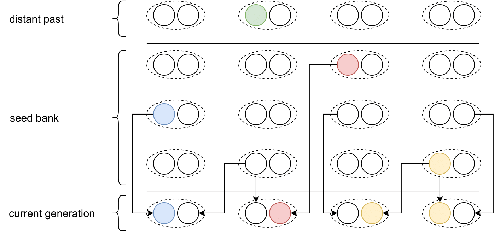
Consistent with this concern, I suggest that you review Figure 1, as this Figure illustrates the forward-in-time two-step process considered in Kaj et al. (2001) who assumed a haploid model, and not a diploid model as in this manuscript. A revised Figure could (should) represent diploid seeds, each seed choosing its two parents from the same generation in the past.
Last, I invite you to consider the following minor comments/suggestions:
Line 5 of the abstract: “signals of selection” -> “signatures of selection” or “footprints of selection”
Line 5 of the abstract: “more narrow” -> “narrower”
Keywords: “weak, dormancy” -> “weak dormancy” (remove the comma)
Lines 15-16: “spatial structure” -> “genetic structure” or “genetic differentiation”
Line 23: “the common ancestor of a population” -> “the common ancestor of a sample of genes from the active population”
Line 49: “representing the populations of size N from the past” -> “representing the past populations of size N”
Lines 79-80: “only the non-dormant lineage is affected by recombination” -> “only the non-dormant lineages are affected by recombination”
Line 127: “indicies” -> “indices”
Line 138: Completing Dr. Jore Koskela’s first comment (see below), the definition of the probability vector $\textbf{Y}^{norm}$ should read: $\textbf{Y}^{norm} = \frac{\textbf{Y}}{\sum_{j=1}^{m} Y_j}$, or: $Y_k^{norm} = \frac{Y_k}{\sum_{j=1}^{m} Y_j}$
Line 154 “Sequantially” -> “sequentially”
Line 187: “As previously stated the simulation process can ran, independently of tskit, but is required when planning to analyze the genealogy” -> “As previously stated the simulation process can be ran independently of tskit, but the latter is required when planning to analyze the genealogy.”
Lines 191-192: “(Figure S1 and Table S1 for empirically sufficient number of calibration generations given for a recombination rate)” -> “(see Figure S1 and Table S1 for characterizing empirically the sufficient number of calibration generations needed for a given recombination rate)”
Line 221: “if it stays at a size of 2N for m consecutive generations“ -> “if its number of copies is 2N for m consecutive generations”
Lines 285-286: “[...] decreasing the value of b (i.e. the longer seeds remain dormant)” -> “[...] decreasing the value of b (i.e., leaving seeds dormant longer)”
Figure 2b: indicate what shaded areas represent (as in Figures 3b and 3c).
Figure 3: The last sentence in the legend (“Dashed-blue lines indicate theoretical expectations of a Ne-scaled population corresponding to a given seed bank strength.”) repeats what is written above (“The blue lines indicate the time to fixation in a population without dormancy but with an effective population size scaled by”), does it not?
Line 331: “(e.g. Figure 4b, 4d and S10)” -> “(e.g., Figures 4b, 4d and S10)”
Figure 4: The legend for (3c) should rather read: “(c) $\pi$ assuming two recombination rates r = 10−7 per bp per generation (c1) and r = 5 × 10⁻⁸ per bp per generation (c2).”
Figure 4: “(b) Normalized $\pi$ as divided by the average neutral branch diversity from (a) using the values 2,000 and 16,000 for b = 1 and b = 0.35, respectively.” What are the values 2,000 and 16,000? (values of what?) It does not seem to relate to a scaling by $\frac{1}{b^2}$, and I am therefore not quite sure to understand how $\pi$ is normalized.
Lines 327-328: “Moreover, stronger dormancy also generates narrower selective sweeps around sites under positive selection which have reached fixation”: when comparing Figures S10 and 4, I would rather conclude that stronger selection (i.e., s = 1 vs. s = 0.2) generates narrower selective sweeps around sites under positive selection (since the rate of dormancy is the same in both Figures). Please, correct the sentence, or be more explicit.
Figure 5: in the legend, (a12,b12) should read (a21,b21) to be consistent with the Figure.
Line 370-372: I would move the sentence “Following the classic procedure to detect sweep [...]” above, since it provides the criteria used to obtain the results from lines 367-370.
Lines 379-380: “We note that there is a much sharper decrease in the rate of detection of false positive sweeps (neutral simulation line in Figure 5) under seed bank compared to the absence of a seed bank.” Do you have any insight about why would that be? It might seem a bit counterintuitive.
I thank you very much for submitting your manuscript to PCI Evol Biol, and I look forward to receiving your revised manuscript.
Best regards,
Renaud Vitalis
, 27 Feb 2023I think this is a thorough paper on a topic which is of both mathematical and biological interest, and the comments I made in the previous round have been fully addressed. I only have two further, superficial comments to add:
1. Page 4, line 137: In the vector Y = (Y_1, ..., Y_m), it looks as if Y_k means the kth entry of Y. However, on the same line Pr(Y_k) seems to stand for the probability of the event that a random variable takes the value k. Do you mean Pr(Y_j = k)?
2. Page 6, line 187: "As previously stated the simulation process can ran..." seems to be missing a "be".
The authors have made substantial efforts to tackle the questions raised by all reviewers, including myself. They corrected some errors in the code and updated the simulation results, they included new analyzes on allele frequency dynamics and sweep detection, and they significantly revised the text and figures of the manuscript. Some clarifications and corrections are still needed but should be very easy to implement.
Line 27, 53 and many others : ‘coalescent’ is the name for the stochastic process describing the genealogy of a sample, so it is correct to talk about the Kingman ‘coalescent’ (for instance). But the events within this process are ‘coalescence’ events, and similary one should talk about ‘coalescence’ rates, ‘coalescence’ times …
L48-50 : Is it unclear what ‘representing the populations of size N from the past’ means.
L85 : ‘a’ Sequentially Markovian Coalescent.
L89-94 : I don’t understand the arguments here. If the fixation time of selected alleles is not multiplied by 1/b² but by a smaller rate, it is smaller than expected and the selection is thus more efficient, not ‘altered’. Similarly at line 97, why do seed banks ‘decrease’ the efficacy of selection. Based on the results of Figure 3, I assume that L91 is maybe wrong and that fixation time is multiplied by a ‘higher’ rate.
L100 : ‘on’ is probably missing between ‘seed bank’ and theta’.
L137 : Yk is a probability, so one should write Y_k=b(1-b)^(k-1), not P(Y_k)=…
L154-156 : I don’t understand where SMC is used, given that simulations are forward in time and SMC is a backward model.
L188 : Is it meant that ‘tskit is required when planning …’ ?
L190 : Since this calibration phase strongly dpends on the population size, it would be better to describe it after introducing the simulated population sizes.
Figure 2, S1 and S8b : Why recording the ‘oldest TMRCA per sequence’ ? This switches the focus from the mean coalescence time to the maximum coalescence time, which probably explains why this quantity depends on the recombination rate (Figure S1).
Line 307 and 311 : I am not sure that 3c is the correct reference here, is it not 3b ?
Line 317 : Is it not rather ‘decreasing b’ ?
Line 328 : ‘S10’ → ‘(Figure S10)’
Line 345 : ‘smooth’ would maybe fit better than ‘sharp’ ?
Line 365 : ‘these variations’
L372-375 : The link between the two sentences is not obvious to me. Decreasing the window size may increase the rate of true positives more than that of false positives, resulting in a higher power for a fixed false positive rate threshold.
Figure 5 : ‘0 generations’ is missing at line 4 of the legend.
L375-376 : It seems to me that these sweeps are already detectable in b21, not only in b22.
L414-417 : A verb is missing in this sentence.
L 425-428 : This sentence is a bit confusing, especially the part ‘which did not compute the probability of fixation of an advantageous allele’.
Figure S3 : The legend says that time is normalized, but it is not clear which normalization is used.
Figure S8 : « =0.35 » is missing in the legend (current text ‘b=1 and b for ... ».
Figure S9 : I don’t understand why Ne*s is 800 for b=1 but 400 for b=0.35. I thought the aim of this analysis was to have the same Ne for both values of b ?
Figure S10 : Same comment as for S9, although I don’t clearly see whether these two figures have the same or different objectives. I note that in Figure S9 the sweep is narrower with b=1, while in S10 it is narrower with b=0.35 : how can we explain this ?
The authors have done an admirable job improving the manuscript, both by addressing my comments and the comments of my fellow reviewers. I have no further comments and believe that it should be recommended by PCI Evol Biol.
DOI or URL of the preprint: https://doi.org/10.1101/2022.04.26.489499
Version of the preprint: 1
Dear Dr. Vitalis,
the following part contains original reviews and suggestions kindly provided by the reviewers and yourself, with an additional reply added from my colleagues and me under each paragraph, hoping to address your points sufficiently. We appreciate the time you take in looking at the manuscript again and apologize for the delay.
Kindly,
Kevin Korfmann
Dear Mr Korfmann,
your manuscript entitled "Weak seed banks influence the signature and detectability of selective sweeps" submitted to PCI Evol Biol has now been examined by four reviewers. All reviewers and I agree that your study is sound, and addresses an interesting and timely question in population genetics: how seed or egg dormancy influences evolutionary dynamics, in particular the fate of advantageous mutations, and the power to detect them. Furthermore, the release of a new simulation tool, which generates SNP data from evolutionary models including weak seed banking and selection, is much appreciated.
Based on the reviews and my own appreciation, I would be glad to consider a revised version of your manuscript for recommendation in PCI Evol Biol, provided you carefully address the reviewers’ points and comments, and provide a point-by-point response to their concerns.
Reply: We thank Dr Vitalis (recommender) and the four reviewers for spending their time to provide in depth reviews and for acknowledging the interesting aspects of our study. We address all points raised by the reviewers. In a nutshell, we have improved and corrected the simulation code, so we have rerun all analyses to demonstrate that all results are consistent with the theoretical expectations, and improve the interpretation of our results. We also run an additional set of analysis to quantify which phase of a sweep is most affected by seed bank. We also perform new analyses to include sweep detection with SweeD (in addition to OmegaPlus) which relies on the SFS signatures. We are sorry for the delay in performing these new analyses, and hope the new revised preprint can be recommended in PCI Evol Biol.
In addition to the reviewers’ comments, I invite you to consider the following points:
My understanding of the model description (section 2.1) is that, each generation, "parents" are picked from a randomly chosen age group (see lines 161-162), and one "gamete" is generated from each of these parents to create a "seed" (haploid model). This wording choice introduces the notion that parents are dormant (i.e., in a non-reproductive stage) rather than seeds. Although I agree that it amounts to the same from a modelling perspective, I wonder whether the text could be clearer by considering, e.g., that each generation parents produce seeds, and that seeds enter a dormant stage at rate (1 – b).
Reply: The description has been modified to clarify this point.
Although the manuscript is overall well-structured and nicely organized, I concur with the reviewers that some of your conclusions could be more clearly stated. For example, the claim made lines 325-326 that "Taken together, the results in Figure 3a, 3b and 3c demonstrate that [weak] selection is slowed down by dormancy", is opposed to the claim made lines 333-334 that "[...] yielding the counter-intuitive result that dormancy enhances the efficiency of [strong] selection compared to genetic drift": (i) it is not clear to me how the latter conclusion is reached from Figure 3; (ii) using different wordings ("slow down", "enhance the efficiency", "magnify", etc.) as synonyms does not help.
Reply: We have now clarified the description of the results by describing more precisely time to fixation and probability of fixation, to avoid unclear statements.
Figures
As the reviewers, I believe that Figures 2-5 (and their legends) could be improved. In addition to reviewers’ comments, I noticed that, in each panel, ticks are missing from the bottom and left axes.
Reply: All figures have been completely revised to include the suggestions from the reviewers.
In Figure 4d: "b 1.0 r 5e-5" should read "b 0.35 r 5e-5". Please provide the effective size for this set of parameter values, for the purpose of comparison with a model without a seed bank (in order to justify the claim lines 353-354 that "the results in Figure 4 cannot be produced by scaling only the effective population size in the absence of dormancy").
Reply: This information is included now in the legend.
Open access
The reviewers appreciated the release of simulation codes on a public repository. However, an anonymous reviewer found it difficult to run the example Jupyter scripts. Please, consider expanding the installation guide, as suggested by this reviewer.
Reply: We have improved the installation guide based on the new sets of codes.
Conflict of interest
The article must contain a "Conflict of interest disclosure" paragraph before the reference section containing this sentence: "The authors of this preprint declare that they have no financial conflict of interest with the content of this article."
Reply: A conflict of interest statement has been added.
Minor points
Line 152: define explicitly the X_parent variable; the multinomial notation is cumbersome and should use vector notations instead. Idem in Equation (2).
Reply: The definition is now on line 137, and we use as suggested the vector notation + multinomial notation alongside a description of the constraints of suitable number spaces.
Cite "Maynard Smith and Haig 1974", instead of "Smith and Haig 1974" (see lines 343, 417, 458, and reference [38]).
Reply: Citation modified.
I thank you very much for submitting your manuscript to PCI Evol Biol, and I look forward to receiving your revised manuscript.
Best regards,
Renaud Vitalis
+++++++++++++++++++++++++++++++++++++++++++++
Review by Guillaume Achaz, 08 Jul 2022 16:41
The ms by Korfmann et al. describes a diploid Wright-Fisher model with seed banking together with a C++ implementation that performs Monte-Carlo simulations. The ms is sound, very clearly written and addresses an interesting question of evolutionary biology. I believe it has the potential to be recommanded by PCI Evol Biol. I nonethless have some suggestions that could help clarifying some of the points discussed by the authors.
Reply: We thank Dr Achaz for his kind comments.
I know realize that there are many points, but they are all easy to fix or be discussed.
:: Main comments ::
- I am unsure the interpretation of the Probability of fixation (Pfix hereafter) is sound. For a sweep in a finite population, there is a drift barrier of low frequency and the fate of the beneficial allele is settled in the first generations. I suspect that with seed dormancy, the probability to leave 0 descendants for the beneficial allele in the m first generations (meaning never leave any descendant) is simply higher. This would be the same for the probability of extinction in general after securing few descendants in the first generations. I am late in my review and only attempted the case of m=2, but this seems doable without much pain for m generations for any kind of distribution. The effect of sampling from several previous generations for each descendant cannot be simply synthesized as "longer time for drift to eliminate the beneficial allele". By some work, using birth and death processes (see specific point on l302 below), I suspect the probability of fixation can be computed with some extra-work (this is not what I expect from the authors in the present article, but it could be worth doing it on a future work).
Reply: The reviewer is correct that it should be doable to perform such theoretical analysis, which we hope to do in the near future. For the time being we first revised and corrected our code as we found a problem in the calculations for the probability of fixation. Our results now agree with previous analytical expectations: the fixation probability is approximately 2hs for all parameter values. Moreover, we analyze in response to reviewer 4 (Dr. Boitard) the dynamics of changes in allele frequency to investigate more precisely the impact of dormancy on the different phases of a sweep dynamics: low allele frequency and intermediate to high frequency. The new results are now shown in Supps Figure S2-4 and discussed.
The fixation time (which should be corrected all along this article by "mean fixation time") is very well approximated for a finite haploid population of size N by
E(Tfix) = 2 ln (N . Pfix +\gamma_e)/s
in a haploid WF model, where \gamma_e is the Euler constant. As the intensity of dormancy (\beta) will enter on Pfix within the log_e, we can immediately see that the relationship will not be trivial. So it does not come as a surprise that there is not simple relationship between beta and E(Tfix). I have not worked the diploid version with h != 0.5, but it may well add a layer of complication adding further complication to the relationship.
Reply: Thank you for pointing this out. We had neglected the non-linear relationship between Tfix and Ne.s, which led to a partial interpretation of the results. An approximated result is found in Koopmann et al. 2017 (equation 19), where it indeed appears that the relationship is not trivial and likely non-linear. We have added the expectations of Tfix to Figure 3, based on the equation above and the diffusion approximation given by Kimura and Ohta (1969) for weaker s, as the above equation does not give reliable results in that range. The time to fixation is actually much higher with dormancy than would be expected for a similar Ne. This has resulted in a change of our take home message: Dormancy makes selection less efficient. This is highlighted by the new Supp Figs (S2-4) where we show that as b decreases and s increases, more time is spent at very low and very high frequencies of the allele under selection with regards to the time spent at intermediate frequencies.
- There is a need to explain how the software OmegaPlus works and what is the value "Omega" for casual (understand lazy) readers that would like to read your article without having the duty of reading the OmegaPlus articles. Just the basic ideas would be a great added value.
Reply: More details and comments about OmegaPlus have been added in the section 2.3 Statistics and sweep detection section (second paragraph)
- Figure 2a, you are plotting average TMRCAs when the recombination rate is >0, right ?
Reply: We simulate 200 DNA sequences of 0.1Mb with recombination. From all the trees of a given simulation run, we use the time of the most ancestral node from the tree containing it as TMRCA. Or said differently, from all the ancestral nodes of a given simulation, we choose the oldest time as TMRCA per sequence. Therefore, when there is no recombination, we obtain one TMRCA per sequence, otherwise under recombination, we retain only the oldest TMRCA per sequence.
:: Specific comments ::
Abstract: l21-22: the sentence about magnifying and lowering selection is especially confusing. If it decreases the Pfix, how could it magnify selection? What "magnify" means here is unclear.
Reply: We acknowledge that our choice of words was confusing and have now streamlined our results description. This particular sentence has been removed.
l31- authors list all sorts of organisms but not fungi... but they produce spores. This is likely due to my ignorance, but I would have guessed that fungi tend to sporulate when the nutriments are less abundant (this is at least true for S cerevisiae and S pombe) and are likely concerned by dormancy.
Reply: Indeed, fungi are well-documented organisms portraying dormancy traits, and we now mention them.
l40-41: buffering mutation rate? What does this mean?
Buffering population size changes, not mutation rate. Added “affecting mutation rates”, to make it more clear.
l80: any intuition on the formula?
Reply: We are not sure which formula the reviewer meant, but guess that it refers to the 1/beta². The intuition in a coalescent framework (see Kaj et al. 2001) is that for two lineages to find a common ancestor, i.e. to coalesce, they need to choose the same parent in the above-ground population, and each have a probability beta to do so because only active lineages can coalesce. Thus the probability that two lineages are simultaneously present in the active population is beta², thus scaling the coalescent rate. This is now included in the next sentence.
l90 : effective population size is always fuzzy. I believe you refer to "inbreeding" population size. It would not cost much too state 'inbreeding effective population size".
Reply: Done, it is now stated in the introduction.
l96: there is an unnecessary ")" in the \theta definition
Reply: Fixed.
l102: "Only one" can be replaced by "The non-dormant" or "The active" or any other more precise wording.
Reply: Changed to “only the non-dormant”
l116 : we read again the "efficacy" of selection. This is confusing. Mean fixation time is longer but at the same time the "efficacy" is increased. What are we measuring then, since mean Tfix is longer and Pfix is smaller? How could it be more efficient?
Reply: Again we apologize for the poor choice of words. When analyzing the time spent in the two “stochastic” phases as well as deterministic phases (see Appendix Figure S2-4), and performing computation of expected fixation times (Figure 3b), we saw that selection is actually less “efficient” compared to a 1/b² rescaled population. This is because the allele spends comparatively longer in the stochastic phases. We adapted the message of the paper, and are more precise now when defining time to fixation or probability of fixation and we avoid using efficiency or efficacy.
l152 + l162 : please define properly X and G. I am not sure parent "1" is the best subscript as it is true for all individuals.
Reply: The section and notations have been revised.
l159: numerator is also clear when written as 1-(1-b)^m (and faster to computer)
Reply: Thank you for the suggestion. It is indeed improving the computational efficiency.
l160: a truncated geometric would be an adequate name for the distribution.
Reply: Changed.
par l163-l171: this implies there is a single chromosome of size 1, but later (par l208-l220) there is a variable map length. So I think Poisson (L\mu) and Poisson (Lr) can be introduced here and L can be defined as the map length. Please mention that a single chromosome is considered.
Reply: We now removed to the notion of map lengths and refer to chromosome or sequence only. We additionally added the simulated sequence length, ranging from 100kb up to 10MB.
l182-l184: As the probability of being chosen is inflated for all generations, it seems to me that the survival probability is overall inflated. So I am not sure whether the sentence is truly correct.
Reply: The description of the model was improved and this sentence modified.
l196-198: not easy to grasp on for someone who doesn't know the arcane of tskit. Can the author provide a sentence to at least get an idea of what is going on?
Reply: Changed. The paragraph has been partly rewritten, to emphasize that one can run the simulations without recording the genealogies, which is the purpose of tskit. The first paragraph of the methods explains why we use tskit (and the general idea). And the last paragraph of the code description paragraph justifies its usage over SLiM.
l200: I believe 5pN is better choice for the burn-in (where p is the ploidy). This stems from Malécot recursion on Heterozygosity that will be almost at equilibrium (to a 1% relative difference) at approximately 5 times the chromosome pool size (N for haploids).
Reply: Many thanks for this insight, and we have now studied this issue carefully and derive an ad hoc burn in time taking into account the dormancy rate. In the first implementation, there was an issue using to small burn-in generations for the high recombination rate. Now we have added an appendix figure S1 showing the absolute TMRCA dependent on the recombination rate to demonstrate that there is sufficient burn in time. Based on experiments of trying different recombination rates, we came up with a an empirically sufficient number of burn-in generations (see Appendix table) to reach theoretical expectations (especially for the neutral diversity background in the sweep figures, i.e. left and right sides of the chromosome). For a recombination rate around 10^-7 - 10^-8, we choose burn-in for 200,000 generations for a population of 500 diploids under b=0.35 dormancy. Choosing such a large number increases substantially the computational time for the large number of simulations we ran, but it was necessary. We now included the rationale for using different burn in times in Figure S1.
par l222-232: For the haploid case, an easy way to condition on fixation is simply to set a random individual at the selected type and attribute the others uniformly as in a regular WF model. I wonder if there would be a similar trick for this case (no fix is required, this is just a hint on how to speed up the simulator for future work).
Reply: Thanks for the idea, sounds interesting indeed.
l236: would it be appropriate to (also) cite Tajima 83 for "Tajima's \pi" (that was noted k in 83)?
Reply: Tajimas 83 citation is added now.
l258 - Is running time also very efficient for s=0.01 or lower s values?
Reply: By now we have rewritten the simulator so that lower selection coefficients can be easily tested. In fact we test in the new version values as low as Ne.s=0.1, corresponding to s=0.0001 and assess the probability and time to fixation.
l292- I think the recombination events are 1 per coalescent tree (in a tree sequence) or NLr/b per coalescent unit.
Reply: Indeed there are 1/b more recombination events per chromosome. The sentence has been modified.
Fig2a - make sure it is 2 in coalescent unit for b=0.
Reply: Yes. We have double-checked and made sure that values are within theoretical expectations. An appendix figure with absolute values has been added additionally.
l 302 - I am not sure the difference comes from the N=500. 1-exp(-2s) is only valid for small s. Another potential derivation is to use the probability of survival of a critical birth-death that starts with 1 individual, who has a Poisson number of descendants (of mean \lambda), leading to 1-Pfix = Exp(- \lambda Pfix ). The dominance may add some complications, though. I believe you used h=1 here ?
Reply: We used h=0.5 as our focal dominance coefficient. A sentence has been added to clarify this. Additionally, the probability of fixation is no longer affected by the germination rate.
Figure 3: please specify the parameters. N, h, range of s.
Reply: Added.
l 327- I don't understand the meaning of this sentence.
Reply: the sentence has been rewritten.
par l329-l334: see main points above.
Reply: the sentences have been rewritten to account for the updated simulator version.
Figure 4.d: what is N for b=0.35?
Reply: corrected.
l404: "a period of 1 / 2 Ne or 1 / 2 Ne s"? What do I don't understand?
Reply: Modified to time to fixation instead of period.
l431-432: see main points above
Reply: Because our results and main conclusions have changed, this is no longer an issue.
+++++++++++++++++++++++++++++
Reviewer 2
This article presents the first analysis of the joint effect of selective sweeps and so-called
weak seed bank dynamics, in which organisms are able to enter a reversible state of metabolic
dormancy lasting a small number of generations. Seed banks are known to slow down genetic
drift, elongate branches in ancestral trees, and increase the effective rate of recombination. The
findings of the article are consistent with these intuitions: fixation probabilities decline, and
the signatures of selective sweeps become narrower but are persist for longer. On the other
hand, predictions derived from deterministic or otherwise simplified models have shown that
the effect of seed banks on the efficiency of selection is subtle [1, 2]. This article presents a
scalable, tskit-based simulation tool for whole genome data under the joint effect of weak
seed banks and selective sweeps, clarifying the applicability of the various predictions to more
realistic models, and shedding light on the nonlinearities involved in the joint effect of dormancy
and selection. The simulation model is a natural extension of the classical Wright–Fisher model.
Given the universality of coalescent models, it is likely that findings are robust to other choices
of individual-based models (at least when suitably rescaled).
The tskit framework is natural for neutral evolution, but more cumbersome for non-neutral
processes since genotypes need to be tracked in addition to ancestral relations. The paper avoids
this issue by tracking genotypes outside the main simulation data structure. Simulation param-
eters are well-chosen, and span a biologically plausible range while remaining computationally
feasible.
The authors have provided their simulator as a GitHub repository sleepy, with brief instal-
lation instructions which I was able to follow. They have also provided an analysis repository,
sleepy-analysis, which I was able to clone. However, despite the installation of the sleepy
package running without errors, the Jupyter scripts in sleepy-analysis were not able to lo-
cate the sleepy method. I am by no means an experienced Jupyter user so may be missing
something obvious, but expanding the installation instructions to include details on how to run
the provided minimal code example would be a good way to improve the accessibility of the
code.
Reply:
A more detailed example notebook has been added. But notably the compilation does not require root privileges, because the executable is not transferred or linked to a directory, where root privilege is required. What we suggest instead is to append the bin directory to your path in the bashrc file:
export PATH=$PATH:/path/to//sleepy/bin
Now, after that is done. It is important to close the window and reopen the terminal window and then open jupyter-lab/notebook
Additionally in the jupyter notebook you can check if sleepy is found by typing bash commands as demonstrated in the example notebook
The simulation outputs consist of a collection of standard population genetic statistics (link-
age disequilibrium, time to most recent common ancestor, etc.), as well as the time until fixation
and an estimator of the fixation probability. The last two are estimated by repeatedly introduc-
ing a selective mutation at a given site until it fixates (rather than goes extinct), and storing
the number of generations until fixation and the number of trials. The latter amounts to esti-
mating the success probability p of a geometric distribution from iid replicates, which is known
to have a p(1 − p)/n bias, but the authors have performed n = 1000 replicates to render the
bias negligible. The simulator is validated using a neutral scenario, for which many expected
values are known analytically.
Overall, the simulations are an interesting catalogue of the joint, nonlinear impact of dor-
mancy and selection on genetic diversity, and of the prospect of detecting sweeps in the presence of dormancy. I agree with the authors that their results are of applied importance in the analysis of many biologically important species, particularly among plants and fungi for which the weak seed bank is a natural model. The main limitations of the results are the assumptions of a
constant population size, and that mutations occur in dormant individuals at the same rate as
in active ones. Both assumptions are discussed and justified by the authors, but the mapping
of diversity patterns arising from dormancy and selection without these assumptions remains
an open task.
Reply: We agree that these models are interesting to explore, but argue that they fall outside the scope of the project, because addressing them would require a substantial number of additional simulations, without adding much novelty to the manuscript.
I have two aesthetic comments on the figures:
1. The neutral line in Figure 3c is effectively invisible. I’m guessing it overlaps almost exactly
with the s = 0.01 line, but it would be useful to say so, or to reformat the plots to make
it obvious.
Reply: We completely redid the plot. Since the average time of fixation of a neutral allele for N=500 is 2000 (2cN with c indicating the ploidy), the neutral allele can be simplify calculated by scaling with 1/b^2. The line corresponds to Ne.s=0.1, i.e. increasing the time to fixation from to 2000 to 32000, which fits the neutral line perfectly now. This is also why we removed it.
2. The colour scheme in Figure 4 also makes it hard to distinguish the different trajectories,
particularly the two blue-hued ones.
Reply: The colour scheme has been changed and all figures are now in high-resolution.
References
[1] L Heinrich, J M ̈uller, A Tellier and D ˇZivkovi ́c. Effects of population- and seed bank
size fluctuations on neutral evolution and efficacy of natural selection. Theor Popul Biol
123:45–69, 2018. [2] D ˇZivkovi ́c and A Tellier. All but sleeping? Consequences of soil seed banks on neutral
and selective diversity in plant species. In Mathematical Modelling in Plant Biology, R
J Morris (ed), Springer, Cham, 2018
+++++++++++++++++++++++++++++++++++
Reviewer 3
Summary
Overall, I think this is an interesting study that leverages existing theory alongside
computational tools, yielding promising results. Ultimately this work should be published, but I
have several minor comments and I believe that the impact of the paper would be
strengthened by addressing them. Most of these comments can be grouped into requests to 1)
elaborate on points the authors made and their connection to population genetic theory and 2)
make alterations to the figures to increase their clarity.
While I am familiar with mathematical models of molecular evolutionary dynamics, I am less
familiar with models of selective sweeps. I have attempted to provide useful feedback and
questions regarding sweeps and their statistics throughout this review.
Major comments
- The authors model the evolution of a recombining population with a seedbank as a
diploid hermaphroditic population. While it may be outside the scope of the manuscript,
it’s worth considering that recombination can be modeled in a more general manner
where there is some probability of recombination per-generation in a haploid
population. Could the authors describe the extent that their model and results can be
extended to haploid populations?
Reply: Previous theoretical results on haploid model (Koopmann et al. 2017, Heinrich et al. 2018) confirm the reviewer’s intuition that the results we obtain are valid for haploids. We expect the same germination rate scaling of the coalescent tree by b^2 and recombination rate scaling of b. Thus, while it would have been possible to design the study using a haploid model, the results are expected to be similar regardless of the chosen ploidy. Initially, when reading how forward simulations work, we started from the work on SLiM by Ben Haller, which is a diploid simulator that inspired the current work. Yet, retrospectively, implementing a haploid model would have likely been easier.
- Line 39: I don’t see why the word “species” is needed here.
Reply: species has been removed.
- Line 200: It would be useful for the unfamiliar reader if the authors made note that the
number of generations they chose for the burn-in corresponds to the coalescent
timescale. My understanding is that this is the timescale of the Kingman coalescent, if so
or if not, please note it in the text.
Reply: This echoes a reply to reviewer 1 (Dr Achaz) above. We added a supplementary figure with the TMRCA times as well as a supplementary table with the burn-in-periods in generations, justifying the large chosen burn-in-period necessary when dealing with recombination and the presence of seed bank.
- Line 204-206: Is there any existing theory that the authors could reference for the order-
of-magnitude timescale required for signatures of a selective sweep to become
detectable?
Reply: The theoretical results are available for classic models (Kim and Stephan (2002) for example), but not in the presence of seed banks. The magnitude is simply 1/b^2, meaning the period that a sweep is potentially detectable is a reflection of the scaling of the coalescent. We added a supplementary figure (Figure S3), to emphasize this.
- Line 219-220: While I understand that an appropriate range of selection coefficients can
be hard to justify, selection coefficients ranging from 0.1-10 seems too high. Even with
the lowest value of the empirical population size (ignoring effective size) of 1,000, the
population-scaled strength of selection is much larger than one for all parameter
combinations (|N*s| >> 1).
Reply: We agree with the reviewer and have now expanded the range from Ne.s=0.1 to Ne.s=100.
I would think that it would be useful to examine signatures
of selective sweeps with and without fixation as the population-scaled strength of
selection (calculated using the effective population size) increases starting below 1 (drift
dominates).
Reply: We wanted to investigate the signatures of sweeps conditioned on fixation as these are the most likely to be detected in real data. Extending to softer sweeps or incomplete sweeps is indeed interesting but increase significantly the parameter space to search and simulate and the result section will be inflated, possibly without a real gain in terms of novelty. We keep this idea in mind for future work on selection and seed banks.
There may be some nuance I’m missing, but as a general pop gen reader
this is the range of parameter values I’d be looking for.-
Line 241–242: It would be helpful for the reader if the authors described the Omega
statistic, how it works, and any additional parameter settings the authors may have
chosen.
Reply: A short description and comments on the choice of parameters have been added.
- Line 271-274: This was a very helpful point, thank you for making it.
Reply: Thank you.
- The strength of selection is not necessarily the key parameter, but rather the
population-scaled strength of selection. Could the authors discuss that quantity in this
sentence instead?
Reply: Thank you for pointing this out. We have included the expectations for the times to fixation without dormancy for different Ne.s, so that the interpretation of our results has changed.
- Line 345-348: This was explained well.
Reply: Thanks
- Fig. 2: a) The recombination rates should be listed in a legend inside the figure. And
what do the boxplots represent? Are they quantile plots? Is so, given that these are
simulation results, it may be more useful for the reader if the spread around the mean
was plotted as 95% confidence intervals.
Reply: We changed the plotting, so the recombination rate is now at the x-Axis and added an explanation about the boxplots in the legend. We additionally plotted the mean and since we changed the axis. Boxplots are likely a sufficient way of representing the data. We agree that if we use the old axis, 95% line plots would have been better. And we further added a supplementary figure with the absolute values. We hope the plots are now clearer.
b) “r2” should be “r2 ” and there should be an
equal sign for “b” in the figure legend. And what are distance bins? Should these be
thought of as base pairs?
Reply: We have changed the legend for figure 2.
- Fig3: a) I do not understand the x axis. Are these selection coefficients ranging from 1 to
5? If so, this is the plot where I’d like to see the population scaled strength of selection
(|Ne *s|) over a logarithmic range of values with |Ne *s| = 1 as a midpoint. The shaded
areas around the lines are not described in the legend and it would be helpful if the
parameter b was included in the figure legend (e.g, b=0.25, b=0.35, etc).
Reply: We are sorry, the axis range was not a good representation of suitable selection coefficients. We completely overhauled the figure now. And are always plotting effective population size scaled values.
b) It would be helpful if the y axis was on a log base 10 scale. Also, “Germination rate, 1/b” should be
written on the x-axis. Again, it would be helpful if “s” was included on the figure legend
(e.g., s=0.01, s=0.1,). C) This is a useful plot, but I think it would drive the take-home
point home is a horizontal line at y=1 was included as a null as dormancy decreases.
Reply: We completely reformatted the figure, to address the points mentioned. And additionally added theoretical expectations based on rescaled N alone in blue.
Also, “Germination rate, 1/b” should be written on the x-axis.
Reply: We completely overhauled the figures, added a population size scaled legend, and added log-scaled subplots and adapted the legend.
- Fig. 4: These are nice plots, but they need some tweaking to help the reader. What does
the shaded area around a line represent? Are these standard errors or 95% CIs. All
parameters in the legends should have equal signs. And “sc” is used in the figure,
whereas “s” is used in the legend. Are these the selection coefficients?
Reply: Figures have been tweaked accordingly and notations are consistent between figures.
- Fig. 5: The y axis could be more informative. Could it be labelled “Probability of
detecting a sweep”? it would be helpful if the parameter under “model” was included in
the figure legend with an equal sign.
Reply: The axis has been changed and the parameters are now part of the legend's title.
Minor comments
- The authors occasionally use the first letter of an author’s first name in in-text citations.
Is there a reason for this?
If not, they should be removed from the revision. I noticed this on lines 42, 84, and 170, for example. I did not count all the occurrences in the
manuscript.
Reply: We changed the citation style to resolve this issue.
- Throughout the manuscript the authors use “e” notation to describe the orders-of-
magnitude of numbers. Could they switch to base-10 notation (e.g., 10-3 instead of 1e-
3?).
Reply: This “e” notation has been removed.
- I may have missed it, but I didn’t see the simulated data repository mentioned in the
manuscript. If it’s not there,
Reply: Indeed the simulated data repository was missing. It is now available on gitlab.
- Lines 24-26: Could bacteria be included here as well? I understand that bacteria are
typically thought of as asexual, but recent research efforts point towards their rate of
recombination being higher than previously thought (Garud, Good et al., 2019; Good,
2020; Sakoparnig et al., 2021).
Reply: Because of the underlying molecular mechanism of how recombination occurs in bacteria versus plants/animals, we are very cautious and do not think that our results are easily transferable. However a recent Bacterial Slimulator code has been developed which could be extended to introduce strong dormancy/seed bank in the future (https://peercommunityjournal.org/articles/10.24072/pcjournal.72/)
- Lines 49: This sentence is somewhat unclear to me. Unless I’m misunderstanding
something, existence of dormancy increases the true T_MRCA in a population, so it will
increase the T_MRCA estimated from a sample from a population. “of a sample or
population“ implies exchangeability between a sample and the true population, which I
don’t think is the authors’ intent.
Reply: Ideally, a sample large enough should have the same TMRCA as the population, so they should be ideally exchangeable. As it may be confusing, we remove the sample part and only leave the population.
- Lines 61-63: I think it’s worth mentioning that the weak seed bank model is also
applicable to cases where the existence of a seed bank is experimentally imposed,
where it is unfeasible for the observer to observe a system over the timescale required
for the strong seed bank effect. This could include bacteria (e.g., Shoemaker et al.,
2022).
Reply: Cool suggestion, thank you. It has been added.
- Lines 74-77: This was well said.
Reply: Thanks.
- Line 100: How do mutation rates work here? Seeds don’t reproduce, so they’re
acquiring mutations at some rate per-unit time (days, years, etc.), whereas the above-
ground plants are acquiring mutations at a rate of per-generation. Are there any rough
estimates of how these rates compare when they have the same units?
Reply: As seeds are essentially just “parents” from previous generations and time is discrete, we have exactly the same rate in the current generation and “seed generation”, which is in units of mutation events per bp per generation. And because of that, we can simply add the mutations to the branches afterwards, if required. There is no need to distinguish a parent that emerged from a seed or from the previous generations when applying the mutation rate. We hope that Figure 1 as well as justifications L.76 clarify this assumption. We choose this definition for convenience of modeling and due to the lack of empirical evidence regarding the empirical mutation rate in seeds per real time unit (days, year…). It could be expected that mutations accumulate in very long dormant seeds compared to short dormant seeds, but again the empirical evidence is so far lacking (and many mutations occurring in seeds maybe deleterious, see argument in Vitalis et al. 2004).
- Line 227-228: Should it be either “frequency of one” or “size of 2N”.
Reply: Modified “to size of”.
- Line 300-302: I’m unsure what the shaded areas are in the referenced figure, but if the
authors resample the simulated data with replacement to obtain 95% CIs, would they
fall within the theoretical prediction? This may allow you to confirm that stochasticity
was a contributing factor.
Reply: This statement was out of date as the updated simulator does not have this issue (the probability of fixation is unaffected by dormancy).
- Line 329-332: “However, when the beneficial allele reaches fixation, the time to
fixation” I do not understand the framing of this sentence. It seems to be implying that there is some non-zero time to fixation once an allele becomes fixed (i.e., all individuals
have the mutation).
Reply: This sentence has been corrected.
- Line 333-334: “yielding the counter-intuitive result that dormancy enhances the
efficiency of selection compared to genetic drift”. I don’t understand what “efficiency”
means here. The plot in Fig. 3c examined the time to fixation with a seedbank relative to
the time to fixation without a seed bank. This ratio seems to increase with germination
rate for all selection coefficients, so I do not see how the notion of “efficiency” fits in
here.
Reply: The sentence was removed, because it was not longer holding true with the updated simulator.
- Line 423: replace “>=” with “≥”
Reply: Fixed
- Line 460: What are the CLR tests?
Reply: Composite likelihood ratio test of SweeD. This sentence has been reformulated and we remove the “CLR-Test” as it was not needed here.
- Line 473: Should “reduce” be plural?
Reply: Fixed.
- Listing 1: Should “analysis of” be “analysis”?
Reply: corrected
- Fig. 1: Do the authors have a version of the figure with higher resolution? In its present
form, the resolution contrasts with the resolution of the PDF, drawing the eye towards
the difference.
Reply: All Figures are high-resolution pdfs now.
- Appendix: In both figures in the appendix, it would be helpful if equal signs were
included for the parameters. It is also unclear what the parameter “d” represents.
Reply: all figures have been adapted.
References
Garud, N. R., Good, B. H., Hallatschek, O., & Pollard, K. S. (2019). Evolutionary dynamics of
bacteria in the gut microbiome within and across hosts. PLOS Biology, 17(1), e3000102.
https://doi.org/10.1371/journal.pbio.3000102
Good, B. H. (2020). Linkage disequilibrium between rare mutations. BioRxiv,
2020.12.10.420042. https://doi.org/10.1101/2020.12.10.420042
Sakoparnig, T., Field, C., & van Nimwegen, E. (2021). Whole genome phylogenies reflect the
distributions of recombination rates for many bacterial species. ELife, 10, e65366.
https://doi.org/10.7554/eLife.65366Shoemaker, W. R., Polezhaeva, E., Givens, K. B., & Lennon, J. T. (2022). Seed banks alter the
molecular evolutionary dynamics of Bacillus subtilis. Genetics, 221(2), iyac071.
https://doi.org/10.1093/genetics/iyac071
++++++++++++++++++++++++++++++++++++++++
Review by Simon Boitard, 24 Jun 2022 10:03
In this study, Kevin Korfmann and colleagues describe a new software for the simulation of genome sequences with weak seed banking, an evolution model that is relevant to many plant, fungi or invertebrate species. This simulation tool exploits the recently developed tskit library, which makes it very efficient. It allows to simulate evolution models including both seed banking and selective sweeps, which had never been done so far. Thanks to this new tool, the authors investigate several important properties of selective sweeps under a weak seed bank model : the fixation probability and fixation time of new beneficial mutations, the genetic diversity patterns around a selective sweep, and the detection power of selective sweeps. Comparing these properties with those of a standard Wright-Fisher model, they conclude that (i) the efficacy of selection is increased by seed banking for strong selection, but not for weak selection ; (ii) the region of reduced diversity around a sweep is narrower for seed bank models ; (iii) past sweep signatures may be detectable for a longer time period in seed bank models.
These new results provide interesting insights on an important evolutionary process, and the new simulation software developed by the authors will certainly be very useful to researchers wishing to test hypotheses or perform simulation based inference under seed bank models. The context of the study and the underlying mathematical models are nicely introduced, and the manuscript is well structured and generally easy to read. However, some of the conclusions could be more clearly phrased or justified and a limited number of additional analyzes could help strengthening them. These suggestions and other minor points are detailed below.
Reply: Thanks to Dr Boitard for his kind words and summary of our work.
Dynamics of alleles under positive selection :
- The general conclusion that seed banks « magnify » the efficacy of selection in the case of strong selection, made for instance lines 411-413, is not obvious to me and should be more carefully justified, or rephrased. For strong selection, the time to fixation is indeed reduced by seed banking (relatively to the time of fixation of neutral alleles), but on the other hand the fixation probability is increased. It would be important to stress that we have here two opposite effects. Similarly, the discussion in section 4.1 is not precise enough concerning the existence of these two opposite effects, because the expression ‘selection is delayed’ is used to describe the effect of seed banks on both fixation time and fixation probability.
Reply: In echo to comment from Dr Achaz, this part has been rewritten/removed, because it was no longer correct. Please see the next comment, too.
- Figure 3 : to illustrate the idea that selection is more efficient with seed banks (l 334-334), panel c could maybe be normalized by the fixation time under neutrality ? To better compare the effect of seed banks on fixation probability and fixation time, it would maybe help to plot panel a as a function of 1/b, with one curve / color per selection coefficient, and possibly to also normalize it by the probability under neutrality ? Finally, panels b/c would be easier to read if the legend for ‘neutral’ evolution would be the top row, so that this comes just before s=0.01 (similarly, the theroretical prediction in the legend of panel a could be the last row).
Reply: We have revised Figure 3 now, and added in theoretical expectation of times to fixation of populations which are rescaled by 1/b². Additionally, we added appendix figures S2-4, showing which phase (stochastic, or deterministic phases) contribute most to the fixation/loss of alleles under seed bank. We also include a percentage figure to describe which phase contributes the most to allele fixation/loss with respect to the selection coefficients. All these new results show that selection is actually less efficient in the seed bank, because the seed spend more time in the stochastic phases, as we initially thought. Now, we can clearly see the scaling of 1/b² for the neutral case and 1/b for strong selection (as expected from Koopmann et al. 2017). Additionally, computational improvements/corrections made it clear that the probability of fixation is unaffected in the seedbank. We hope by adding all those new figures, as well as theoretical expectations, our message is clearer now.
- Besides these clarifications in the text and in Figure 3, one way to reach a global conclusion on the influence of seed banks on selection dynamics could be to compute the expected number of fixation events per time unit, which would account for both the frequency and the speed of sweep events.
Reply: Thanks for the suggestion. To reach a global conclusion and provide better evidence, we put substantial effort into deciphering the individual contribution of each phase (stochastic, deterministic) to the lengthening of the seed bank. We also include a percentage contribution figure (Figure S4), showing which phase contributes the most of the time spent to reach fixation, indicating that seed banks actually tend to lengthen the stochastic phase. Additionally, we added theoretical expectations in blue (Figure S3) to investigate our initial impression of “more efficient” selection compared to a rescaled population size, which turned out not to be true. So we tone down our conclusion here and revise our initial idea from Koopmann et al. (2017).
Genetic diversity patterns around a sweep :
- l 341-345 : it is clear from Figure 4 that the sweep window is reduced by seed banks, but the interpretation of this result is not so obvious to me. While effective recombination rate is indeed higher with seed banks, fixation time is also shorter (cf section 3.3) so there are fewer recombination opportunities during the sweep (in classical models of selective sweeps, the probability to escape the sweep is related to the product r*tau, where r is the recombination rate and tau the duration of the sweep). I would be interested to have the authors’ feedback on this point.
Reply: We now include a description of this effect along with Figure 4. We note that the new results show less of a difference in the width of a sweep signature between seed bank and absence of seed bank compared to the previous version (see also Fig S10).
- l 345-348 : I don’t understand the rationale here. Should we relate explanation 1) to absolute diversity and explanation 2) to relative diversity ?
Reply: This part has been rewritten. Relative diversity refers to the scaling by 1/b², which can easily be accounted for by scaling the population size by that factor.
- l 354-356 : the observation that no model without seed bank can mimic the genomic patterns of a specific model with seed bank is very interesting ; nice idea !
Reply: Thanks.
- l 368 : « narrower » is exact but « sharper » is not obvious, when looking at the normalized curves of Figure 4b.
Reply: We have added appendix figure S10 to make this effect more apparent.
Detection of selective sweeps :
- Linkage disequilibrium is one of the possible approaches to detect hard selective sweeps. Another very common one is to look at the SFS, as mentionned by the authors in the discusion (software Sweed). Comparing this approach with OmegaPlus on the data already simulated would strenghten the conclusions of the study.
Reply: We have now added a SweeD analysis.
- The comparison between models at lines 380-398 seems a bit approximative. This could easily be solved by indicating the exact detection threshold associated to 10% false positives on each panel of Figure 5 (the x axis of panels b/d could be rescaled to focus on the left part on the graph).
Reply: The figure has been replaced. In the new Figure, we indicated the 5% threshold with vertical dotted lines.
- l 471-474 : there are a number of claims here that would really require more justification, for instance with precise references to previous studies. None of these claims is really intuitive to me.
Reply: This section has been rewritten and streamline, and these sentences were removed.
Model definition :
- l 153 & 164 : in order to maintain a population of N diploids, I suppose that each sampled individual actually contributes two gametes, not one.
Reply: We sample two times N individuals, each contributing one gamete, or part of a gamete (in the case of recombination.) We added lines 121-122 to clarify this point.
- Equation (1) : if I refer to the last line, Y_i is a probability, not a stochastic variable. To be consistent with this notation, the first line should be something like Y_i=P(Generation=k_i)=…
Reply: corrected (line L130).
- Equation (2) : the first parameter of the multinomial is the number of draws; I think this is 1 here, not m.
Reply: Exactly, it should have been 1 indeed. In the new rewritten version, it is now N because we draw a N dormant generation, one for each parent.
Minor points :
- l 14 : « means » → « implies »
Reply: Changed.
- l 21-22 : this is an important conclusion of the study so I would avoid the use of ‘respectively’ within parentheses and write a specific sentence or sub-sentence for each type of selection.
Reply: it has been rewritten.
- l23-24 : In section 3.4 the authors show that selective sweeps are detected for longer time with seed banks, but explain it by the fact that new mutations need longer time to accumulate from the end of the sweep. The link with recombination rate made in this sentence is thus not justified.
Reply: The sentence has been corrected, the longer detectability is due to the rescaling of the ARG, not the increased recombination rate.
- l 62 : the formulation « a few ... compared to ... » is not correct.
Reply: Modified.
- l 65 : « as we ... » → « in order to » ?
Reply: corrected.
- l 220 : I suppose that 1.1 should be 1 ?
Reply: We specifically test dominance coefficients of 0.1, 0.5 and 1.1, representing recessive, co-dominant and overdominant beneficial mutations.
- l 248 : what is the meaning of these parameters ? Actually, maybe a few lines about how OmegaPlus works would be helpful.
Reply: this has been addressed now.
- l 250-251 : this last sentence is a bit confusing, because no previous reference was done to the notion of « recovery scenario ».
Reply: The sentence has been rephrased.
- l 308-309 : The first of these two sentences could be removed, to my opinion it makes things more complex than they actually are ; the important point here is that the ratio of the probabilities with and without seed banks decreases for stronger selection.
Reply: This sentence has been removed since the probability of fixation is not affected anymore.
- l 329-332 : Maybe say clearly here than fixation is faster than expected based on 1/b².
Reply: This section has been rewritten in light of new results, as the seed bank is not faster compared to a population rescaling but actually slower (see blue expectation lines in Figure 3).
- l 364 : « as a result of » → « based on »
Reply: corrected.
- l 366-367 : Figure 4 does not explore point 2 (influence of the time elapsed since the sweep).
Reply: We added appendix Figure S5 to explore the time since the sweep by plotting the sweep signatures from 1,000 – 16,000 generations after the fixation has occurred. This shows that sweeps can indeed be detected for much longer, when there is a seed bank.
, posted 20 Jul 2022Dear Dr Korfmann,
your manuscript entitled "Weak seed banks influence the signature and detectability of selective sweeps" submitted to PCI Evol Biol has now been examined by four reviewers. All reviewers and I agree that your study is sound, and addresses an interesting and timely question in population genetics: how seed or egg dormancy influences evolutionary dynamics, in particular the fate of advantageous mutations, and the power to detect them. Furthermore, the release of a new simulation tool, which generates SNP data from evolutionary models including weak seed banking and selection, is much appreciated.
Based on the reviews and my own appreciation, I would be glad to consider a revised version of your manuscript for recommendation in PCI Evol Biol, provided you carefully address the reviewers’ points and comments, and provide a point-by-point response to their concerns.
In addition to the reviewers’ comments, I invite you to consider the following points:
My understanding of the model description (section 2.1) is that, each generation, "parents" are picked from a randomly chosen age group (see lines 161-162), and one "gamete" is generated from each of these parents to create a "seed" (haploid model). This wording choice introduces the notion that parents are dormant (i.e., in a non-reproductive stage) rather than seeds. Although I agree that it amounts to the same from a modelling perspective, I wonder whether the text could be clearer by considering, e.g., that each generation parents produce seeds, and that seeds enter a dormant stage at rate (1 – b).
Although the manuscript is overall well-structured and nicely organized, I concur with the reviewers that some of your conclusions could be more clearly stated. For example, the claim made lines 325-326 that "Taken together, the results in Figure 3a, 3b and 3c demonstrate that [weak] selection is slowed down by dormancy", is opposed to the claim made lines 333-334 that "[...] yielding the counter-intuitive result that dormancy enhances the efficiency of [strong] selection compared to genetic drift": (i) it is not clear to me how the latter conclusion is reached from Figure 3; (ii) using different wordings ("slow down", "enhance the efficiency", "magnify", etc.) as synonyms does not help.
Figures
As the reviewers, I believe that Figures 2-5 (and their legends) could be improved. In addition to reviewers’ comments, I noticed that, in each panel, ticks are missing from the bottom and left axes.
In Figure 4d: "b 1.0 r 5e-5" should read "b 0.35 r 5e-5". Please provide the effective size for this set of parameter values, for the purpose of comparison with a model without a seed bank (in order to justify the claim lines 353-354 that "the results in Figure 4 cannot be produced by scaling only the effective population size in the absence of dormancy").
Open access
The reviewers appreciated the release of simulation codes on a public repository. However, an anonymous reviewer found it difficult to run the example Jupyter scripts. Please, consider expanding the installation guide, as suggested by this reviewer.
Conflict of interest
The article must contain a "Conflict of interest disclosure" paragraph before the reference section containing this sentence: "The authors of this preprint declare that they have no financial conflict of interest with the content of this article."
Minor points
Line 152: define explicitly the X_parent variable; the multinomial notation is cumbersome and should use vector notations instead. Idem in Equation (2).
Cite "Maynard Smith and Haig 1974", instead of "Smith and Haig 1974" (see lines 343, 417, 458, and reference [38]).
I thank you very much for submitting your manuscript to PCI Evol Biol, and I look forward to receiving your revised manuscript.
Best regards,
Renaud Vitalis
The ms by Korfmann et al. describes a diploid Wright-Fisher model with seed banking together with a C++ implementation that performs Monte-Carlo simulations. The ms is sound, very clearly written and addresses an interesting question of evolutionary biology. I believe it has the potential to be recommanded by PCI Evol Biol. I nonethless have some suggestions that could help clarifying some of the points discussed by the authors.
I know realize that there are many points, but they are all easy to fix or be discussed.
:: Main comments ::
- I am unsure the interpretation of the Probability of fixation (Pfix hereafter) is sound. For a sweep in a finite population, there is a drift barrier of low frequency and the fate of the beneficial allele is setelled in the first generations. I suspect that with seed dormancy, the probability to leave 0 descendants for the beneficial allele in the m first generations (meaning never leave any descendant) is simply higher. This would be the same for the probability of extinction in general after securing few descendants in the first generations. I am late in my review and only attempted the case of m=2, but this seems doable without much pain for m generations for any kind of distribution. The effect of sampling from several previous generations for each descendant cannot be simply synthesized as "longer time for drift to eliminate the beneficial allele". By some work, using birth and death processes (see specific point on l302 below), I suspect the probability of fixation can be computed with some extra-work (this is not what I expect from the authors in the present article, but it could be worth doing it on a future work).
- The fixation time (which should be corrected all along this article by "mean fixation time") is very well approximated for a finite haploid population of size N by
E(Tfix) = 2 ln (N . Pfix +\gamma_e)/s
in a haploid WF model, where \gamma_e is the Euler constant. As the intensity of dormancy (\beta) will enter on Pfix within the log_e, we can immediately see that the relationship will not be trivial. So it does not come as a surprise that there is not simple relationship between beta and E(Tfix). I have not worked the diploid version with h != 0.5, but it may well add a layer of complication adding further complication to the relationship.
- There is a need to explain how the software OmegaPlus works and what is the value "Omega" for casual (understand lazy) readers that would like to read your article without having the duty of reading the OmegaPlus articles. Just the basic ideas would be a great added value.
- Figure 2a, you are plotting average TMRCAs when the recombination rate is >0, right ?
:: Specific comments ::
Abstract: l21-22: the sentence about magnifying and lowering selection is especially confusing. If it decreases the Pfix, how could it magnify selection? What "magnify" means here is unclear.
l31- authors list all sorts of organisms but not fungi... but they produce spores. This is likely due to my ignorance, but I would have guessed that fungi tend to sporulate when the nutriments are less abundant (this is at least true for S cerevisiae and S pombe) and are likely concerned by dormancy.
l40-41: buffering mutation rate? What does this mean?
l80: any intuition on the formula?
l90 : effective population size is always fuzzy. I believe you refer to "inbreeding" population size. It would not cost much too state 'inbreeding effective population size".
l96: there is an unnecessary ")" in the \theta definition
l102: "Only one" can be replaced by "The non-dormant" or "The active" or any other more precise wording.
l116 : we read again the "efficacy" of selection. This is confusing. Mean fixation time is longer but at the same time the "efficacy" is increased. What are we measuring then, since mean Tfix is longer and Pfix is smaller? How could it be more efficient?
l152 + l162 : please define properly X and G. I am not sure parent "1" is the best subscript as it is true for all individuals.
l159: numerator is also clear when written as 1-(1-b)^m (and faster to computer)
l160: a truncated geometric would be an adequate name for the distribution.
par l163-l171: this implies there is a single chromosome of size 1, but later (par l208-l220) there is a variable map length. So I think Poisson (L\mu) and Poisson (Lr) can be introduced here and L can be defined as the map length. Please mention that a single chromosome is considered.
l182-l184: As the probability of being chosen is inflated for all generations, it seems to me that the survival probability is overall inflated. So I am not sure whether the sentence is truly correct.
l196-198: not easy to grasp on for someone who doesn't know the arcane of tskit. Can the author provide a sentence to at least get an idea of what is going on?
l200: I believe 5pN is better choice for the burn-in (where p is the ploidy). This stems from Malécot recursion on Heterozygosity that will be almost at equilibrium (to a 1% relative difference) at approximately 5 times the chromosome pool size (N for haploids).
par l222-232: For the haploid case, an easy way to condition on fixation is simply to set a random individual at the selected type and attribute the others uniformly as in a regular WF model. I wonder if there would be a similar trick for this case (no fix is required, this is just a hint on how to speed up the simulator for future work).
l236: would it be appropriate to (also) cite Tajima 83 for "Tajima's \pi" (that was noted k in 83)?
l258 - Is running time also very efficient for s=0.01 or lower s values?
l292- I think the recombination events are 1 per coalescent tree (in a tree sequence) or NLr/b per coalescent unit.
Fig2a - make sure it is 2 in coalescent unit for b=0.
l 302 - I am not sure the difference comes from the N=500. 1-exp(-2s) is only valid for small s. Another potential derivation is to use the probability of survival of a critical birth-death that starts with 1 individual, who has a Poisson number of descendants (of mean \lambda), leading to 1-Pfix = Exp(- \lambda Pfix ). The dominance may add some complications, though. I believe you used h=1 here ?
Figure 3: please specify the parameters. N, h, range of s.
l 327- I don't understand the meaning of this sentence.
par l329-l334: see main points above.
Figure 4.d: what is N for b=0.35?
l404: "a period of 1 / 2 Ne or 1 / 2 Ne s"? What do I don't understand?
l431-432: see main points above
, 06 Jun 2022In this study, Kevin Korfmann and colleagues describe a new software for the simulation of genome sequences with weak seed banking, an evolution model that is relevant to many plant, fungi or invertebrate species. This simulation tool exploits the recently developed tskit library, which makes it very efficient. It allows to simulate evolution models including both seed banking and selective sweeps, which had never been done so far. Thanks to this new tool, the authors investigate several important properties of selective sweeps under a weak seed bank model : the fixation probability and fixation time of new beneficial mutations, the genetic diversity patterns around a selective sweep, and the detection power of selective sweeps. Comparing these properties with those of a standard Wright-Fisher model, they conclude that (i) the efficacy of selection is increased by seed banking for strong selection, but not for weak selection ; (ii) the region of reduced diversity around a sweep is narrower for seed bank models ; (iii) past sweep signatures may be detectable for a longer time period in seed bank models.
These new results provide interesting insights on an important evolutionary process, and the new simulation software developed by the authors will certainly be very useful to researchers wishing to test hypotheses or perform simulation based inference under seed bank models. The context of the study and the underlying mathematical models are nicely introduced, and the manuscript is well structured and generally easy to read. However, some of the conclusions could be more clearly phrased or justified and a limited number of additional analyzes could help strengthening them. These suggestions and other minor points are detailed below.
Dynamics of alleles under positive selection :
- The general conclusion that seed banks « magnify » the efficacy of selection in the case of strong selection, made for instance lines 411-413, is not obvious to me and should be more carefully justified, or rephrased. For strong selection, the time to fixation is indeed reduced by seed banking (relatively to the time of fixation of neutral alleles), but on the other hand the fixation probability is increased. It would be important to stress that we have here two opposite effects. Similarly, the discussion in section 4.1 is not precise enough concerning the existence of these two opposite effects, because the expression ‘selection is delayed’ is used to describe the effect of seed banks on both fixation time and fixation probability.
- Figure 3 : to illustrate the idea that selection is more efficient with seed banks (l 334-334), panel c could maybe be normalized by the fixation time under neutrality ? To better compare the effect of seed banks on fixation probability and fixation time, it would maybe help to plot panel a as a function of 1/b, with one curve / color per selection coefficient, and possibly to also normalize it by the probability under neutrality ? Finally, panels b/c would be easier to read if the legend for ‘neutral’ evolution would be the top row, so that this comes just before s=0.01 (similarly, the theroretical prediction in the legend of panel a could be the last row).
- Besides these clarifications in the text and in Figure 3, one way to reach a global conclusion on the influence of seed banks on selection dynamics could be to compute the expected number of fixation events per time unit, which would account for both the frequency and the speed of sweep events.
Genetic diversity patterns around a sweep :
- l 341-345 : it is clear from Figure 4 that the sweep window is reduced by seed banks, but the interpretation of this result is not so obvious to me. While effective recombination rate is indeed higher with seed banks, fixation time is also shorter (cf section 3.3) so there are fewer recombination opportunities during the sweep (in classical models of selective sweeps, the probability to escape the sweep is related to the product r*tau, where r is the recombination rate and tau the duration of the sweep). I would be interested to have the authors’ feedback on this point.
- l 345-348 : I don’t understand the rationale here. Should we relate explanation 1) to absolute diversity and explanation 2) to relative diversity ?
- l 354-356 : the observation that no model without seed bank can mimic the genomic patterns of a specific model with seed bank is very interesting ; nice idea !
- l 368 : « narrower » is exact but « sharper » is not obvious, when looking at the normalized curves of Figure 4b.
Detection of selective sweeps :
- Linkage disequilibrium is one of the possible approaches to detect hard selective sweeps. Another very common one is to look at the SFS, as mentionned by the authors in the discusion (software Sweed). Comparing this approach with OmegaPlus on the data already simulated would strenghten the conclusions of the study.
- The comparison between models at lines 380-398 seems a bit approximative. This could easily be solved by indicating the exact detection threshold associated to 10% false positives on each panel of Figure 5 (the x axis of panels b/d could be rescaled to focus on the left part on the graph).
- l 471-474 : there are a number of claims here that would really require more justification, for instance with precise references to previous studies. None of these claims is really intuitive to me.
Model definition :
- l 153 & 164 : in order to maintain a population of N diploids, I suppose that each sampled individual actually contributes two gametes, not one.
- Equation (1) : if I refer to the last line, Y_i is a probability, not a stochastic variable. To be consistent with this notation, the first line should be something like Y_i=P(Generation=k_i)=…
- Equation (2) : the first parameter of the multinomial is the number of draws; I think this is 1 here, not m.
Minor points :
- l 14 : « means » → « implies »
- l 21-22 : this is an important conclusion of the study so I would avoid the use of ‘respectively’ within parentheses and write a specific sentence or sub-sentence for each type of selection.
- l23-24 : In section 3.4 the authors show that selective sweeps are detected for longer time with seed banks, but explain it by the fact that new mutations need longer time to accumulate from the end of the sweep. The link with recombination rate made in this sentence is thus not justified.
- l 62 : the formulation « a few ... compared to ... » is not correct.
- l 65 : « as we ... » → « in order to » ?
- l 220 : I suppose that 1.1 should be 1 ?
- l 248 : what is the meaning of these parameters ? Actually, maybe a few lines about how OmegaPlus works would be helpful.
- l 250-251 : this last sentence is a bit confusing, because no previous reference was done to the notion of « recovery scenario ».
- l 308-309 : The first of these two sentences could be removed, to my opinion it makes things more complex than they actually are ; the important point here is that the ratio of the probabilities with and without seed banks decreases for stronger selection.
- l 329-332 : Maybe say clearly here than fixation is faster than expected based on 1/b².
- l 364 : « as a result of » → « based on »
- l 366-367 : Figure 4 does not explore point 2 (influence of the time elapsed since the sweep).
