While the manuscript has improved a lot and there is a lot to like, there still are some issues that need addressing.

While I’m still not entirely convinced by the simulations that are still run for a very small number of generations (but where the allele frequencies are now at least drawn from a beta distribution with alpha=beta=0.5, instead of a uniform distribution), I am willing to compromise on this. The main reason is that given the same sequencing effort, popGWAS always outperformed iGWAS in the same data sets, which is indeed the main selling point of this manuscript (but also iGWAS cannot be used for poolseq data). Thus, whatever shortcomings there are with the simulations, I cannot see how any of them could bias the results in favor of popGWAS.

However, the only information about this iGWAS I can find in the manuscript is on L.325: “… a traditional linear GWAS on a random sample of individuals from all subpopulations was performed for all simulation scenarios ...”. If this is the case, I am not surprised that it did not perform in par with popGWAS, since the iGWAS seemingly did not even attempt to control for any relatedness in the data for instance by including relatedness as a random effect, which is I consider to be a bare minimum (for instance using EMMAX).

Also, it was argued that popGWAS is not sensitive to p-value inflation (L.662-), but for comparison, the levels of p-value inflation were never reported for the iGWAS results nor any attempts to control this (if present). I’m still quite confident that popGWAS can outperform iGWAS but before these shortcomings are addressed, I cannot know for sure.

Furthermore, I’m not convinced that a mean lambda of 1.27 (ranging between 1-1.99, L.440) can be interpreted as no p-value inflation, since the threshold is generally assumed to be 1.1. This is not that much of an issue in the simulations, mainly because the performance was assessed by considering the proportion of true positive loci (TPL) above a given quantile, not a fixed threshold. However, in empirical data, the -log10(P) would, on average, have to be 1.27x higher, provided genomic control was used, which may be the difference between many TPL being significant or not in empirical data.

Perhaps more importantly, SNPs are assumed to represent haplotypes, thus the QTN are assumed to be 100% correlated with the SNPs in the simulated data. This is rarely the case in and to ensure that at least one SNPs is 100% (or at least close to) associated with a QTN (as in the simulations), much higher SNP densities are needed in empirical data for a given level of “LD-structure”. In other words, the ratio between QTN (or SNPs strongly associated with them) and neutral loci randomly sampled in the genome are likely to be much lower in empirical data compared to the simulations making corrections for multiple testing much more taxing (there will many more chances of neutral loci to also be as differentiated as SNPs highly correlated with the QTN or the QTN themselves). This does not take anything away from the fact the popGWAS performed better than iGWAS (but see above), but could be a reason why popGWAS may not be as powerful in empirical data as implied in the manuscript, which should be addressed in the discussion.

One reason p-value inflation was not an issue for popGWAS was the overall high levels of migration between sub-populations (a minimum of 5 migrants per generation), and in addition the simulations were not run for enough generations for population structuring to come into effect (L. 416). Indeed, it seemed that Fst did not exceed much beyond 0.07 in any of the simulations (L. 669), which I still consider to be very low for many species and populations in the wild, and a level that I do not think would lead to much p-value inflation in the iGWAS data either (which is why I would like to see them reported).

Perhaps the biggest weakness of popGWAS in this context is the fact that it relies on some level of “parallelism” (as accurately pointed out on L. 668-692) so migration cannot be too low, which is perhaps the reason why lower levels of migration were not tested. And, as I already pointed out in the previous review, the fact that the simulation started from a common pool of alleles with selection being imposed on the populations before population structuring has reached its full effect gives higher chances of parallelism than would be expected for a given level of gene flow in the wild.

The fact that these the simulations are not at equilibrium is also not an “advantage” as explicitly implied on L. 613-617, since the kind of non-equilibrium that was present in the simulations are highly unrealistic relative to the types of non-equilibrium conditions that can be expected in the wild (population size changes, range expansions etc.).

Furthermore, contrary to what is implied (L.668), many of these limitations are not unique to popGWAS but are expected to affect iGWAS performance as well – QTL involved controlling the same traits across larger number of populations/geographic ranges will overall be more correlated with habitat regardless of how this association is tested.

Ideally, I would therefore want to see that the simulations were run until migration-drift equilibrium BEFORE selection is imposed. Given this, the limits of popGWAS may be apparent already with the, in my opinion, “high” levels of migration so far tested. If not, I would also like to have a level of migration that gives an overall Fst of at least 0.1-0.2, though even higher levels are of course not rare in the wild.

I still do not understand what is meant by the “phenotypic plasticity” parameter (e.g. L. 505). Since “phenotypic plasticity” is not explained anywhere in the text, from the context I assume this is the same as environmental variance, but there is a large difference between these two – plasticity is predictable, whereas environmental variance is not. I think I mentioned this in the first review as well.

Lastly, the idea that “…complex traits are influenced by a few dozen genes that are mechanistically directly involved in their expression, but often also by numerous, if not almost all other genes as well…” is important but not commonly known (and perhaps a bit controversial) and requires thus some more explanation (L. 45-47).
 
 
 

The author made a very thorough job addressing both reviewers comments. I think that the new simulations to compare popGWAS to stablished GWAS-like methods is a great contribution to the discussion regarding the strengths, weaknesses, and releveance of the proposed method. 

I think the current manuscript is rigorous, clear, and will be an important contribution to the community.

 The manuscript “On the potential for GWAS with phenotypic population means and allele-frequency data (popGWAS)” describes a simple method correlating population mean phenotypic values against population mean allele frequencies to identify putative causal nucleotides underlying traits of interest. The principle is the same as in GWAS but using populations, as opposed to individuals, as sampling units. The benefit of this (relative to regular GWAS), is the fact that sequencing (namely PoolSeq) and phenotyping (bulk phenotyping) is cheaper and easier for populations compared to individuals. In addition, by focusing on population, the variance around the phenotypic means is decreased potentially increasing the power of this method when heritability is low (high environmental variance). This approach is somewhat analogous to outlier analyses/genome scan approaches where associations between genotypes and phenotypes are tested indirectly by assuming different habitats have predictably different phenotypic means. Here the focus is also on populations/habitats rather than the individuals, albeit typically these approaches are not readily applicable for PoolSeq data. It is for instance well known that studies of parallel evolution (where similar phenotypic differences are predictably found across different habitats or environmental gradients across a species distribution range) are particularly powerful of disentangling the effects of natural selection from neutral processes such as genetic drift as a source of allele frequency differences between populations (e.g. Johannesson K. 2001. Trends Ecol Evol 16:148–153). 
 
This the premise of this approach is tested in simple forward in time Wright-Fisher simulations, with initial allele frequencies for the ancestral population drawn from uniform distribution with range [0.1,0.9]. From this, sub-populations (500 individuals each) were colonized, each with phenotypic optima drawn from a normal distribution. The allelic effect sizes (for a varying number of loci) were drawn from different distributions. The subpopulations were then allowed to evolve for 2-50 generations, which, in the absence of migration between the subpopulations, resulted in different degree of population structuring between them (due to genetic drift).
 
Overall, the author reported high statistical power to detect phenotype x genotype associations in their simulations particularly when the number of causal loci was low and many populations were sampled, even when heritability was as low as ~30%. Promisingly, reasonable statistical power was also detected for moderately polygenic traits (up to~100).
 
Given the simulations, these results are not surprising for several reasons. We know that rapid adaptation in nature is highly dependent on standing genetic variation. However, in structured populations (the norm in natural populations) this variation is likely to differ between different geographic regions. Thus, what set of alleles are available for adaption (e.g. when colonising new habitats or when the environment changes) can greatly differ from population to population. In the simulation presented in this manuscript, however, the initial allele frequency was the same for all populations (giving each the same probability of having the same set alleles available for adaptation). Furthermore, the initial allele frequencies were drawn from a uniform distribution, while allele frequencies in natural populations (i.e. populations reasonably close to mutation-drift equilibrium) are typically highly skewed towards low frequency variants (further reducing the chance that all populations have access to the same ancestral pool of adaptive alleles in the wild). 
 
There was also a clear trend towards lower statistical power with increasing number of generations of adaptation (Fig. 4D), but the populations were only allowed to adapt for up to 50 generations. These circumstances, i.e. immediate colonization of populations form the same pool of ancestral genetic variation (with unnaturally high numbers of medium frequency alleles) that are allowed to adapt for only 50 generations is the type of scenario where the proposed approach is likely to perform well. Unfortunately, this is also a very unrealistic scenario in natural populations. In the least, the simulations should include some form of a burn-in to allow allele frequencies to reach mutation-drift equilibrium, ideally with different levels of population structuring in the ancestral population and the populations should be allowed to evolve for much longer than 50 generations (and instead allowing different levels of gene flow between them), before any conclusions can be drawn from this study.
 
The test is based on a simple linear regression performed independently for each SNP. From the GWAS literature, we know that population structuring lead to false associations (two populations that differ in phenotype may also differ at neutral loci due to genetic drift), such that great care is always taken to control for this. There are two major ways to achieve this. One is to either include relatedness as a random effect or add population (or PC coordinates) as a co-variate. The other is to perform genomic control to account any residual p-value inflation. Notably, residual p-value inflation may exist even if relatedness is otherwise accounted for (it may not have succeeded to account for everything), and should always be performed. Thus, in all association studies/outlier analyses/genome scans I expect to see some quantile-quantile plots of expected (uniform distribution with range [0,1]) vs. observed -log10 p-values. P-value inflation exist when the slope of a linear regression of these data points is >>1 and genomic control is simply dividing the observed -log10 values by this slope. Without seeing these plot, it is not clear whether p-value inflation exists in the data from the simulations. In more realistic simulations (as suggested above) certainly some level of p-value inflation is expected and would need to be accounted for.
 
The novelty of this approach is that there currently does not exist any method that can utilise PoolSeq data to test for genotype x phenotype associations and as such I would certainly want to see this method tested with more realistic simulations (and ideally also complemented with empirical data as hinted by the author). I expect it to perform similar to other outlier methods out there with the benefit that this is specifically tailored for PoolSeq data (I do not expect it to do well on polygenic traits, but this is perfectly fine). However, seeing as this method is so related to standard GWAS, the knowledge from this field should be utilised better, notably by showing to what extent the approach is susceptible for p-value inflation and then, in the least perform GC (which will reduce false positive rates but also power), but ideally directly control for relatedness e.g. by including relatedness as a random effect, which is expected to reduce false positive rates but not statistical power (at least not to the same extent as GC). As an example, in Fang et al (2021,Mol Biol Evol 38:msab144) such an approach (EMMAX) was successfully used to teste for association between genotype and habitat treated as a binary trait.
 
Some minor comments (in no particular order): 
In the abstract there is no hint on what the test is based on, only how it performs. The title gives some idea, but not enough to be of any help when reading the abstract.
 
I believe that the “phenotypic plasticity parameter“ used in this study is simply environmental variance. Phenotypic plasticity implies a genotype x environment interaction which was, to my understanding, not tested here.
 
L318 “The number of effectively independently evolving loci in a population depends on genome size, effective population size (including all factors that affect it locally and globally) and LD structure”. It is not clear what LD structure means. I my view, all the cited processes effect LD structure so it should not be mentioned as a separate process here.
 
The proposed method only performed well when genome size was small (the number of independently segregating loci in the simulations) and/or the number of sampled populations was large. In large(ish) outbreeding natural populations LD typically declines relatively quickly such that likely >>100.000 (the largest genome size simulated here) SNPs are typically required for the sampled loci to be in sufficiently high LD with the causal loci of interest for them to be useful, especially for polygenic traits. Thus, even if similar performance as presented here can be replicated in more realistic simulations (see above), it seems the proposed method still relies on a large sample size to detect anything but SNPs with large or medium effect sizes (on par with most outlier methods/genome scans approaches that I’m aware of which is not a problem, see above).
 
Given the parallels with methods used to detect parallel/convergent evolution, I’m surprised that this is not discussed more. In particular, the simulations used in this literature are typically much more realistic (e.g. Fang et al. 2020. Nat Ecol Evol 4:1105–1115, Kemppainen et al. 2021. Mol Ecol).
 
L233 “For the assessment of the effect of population structure, the subpopulations could evolve in complete isolation from each other for predetermined number of generations…”  I think it is a bit misleading to consider the number of generations of adaptation in isolation as a proxy for “population structure”. Population structure implies some level of migration-mutation-drift balance in a meta-population setting and the level of population structure should then be modelled by different levels of migration/dispersal. 
 
I am not aware of the F1-score, and I would be grateful for some more information about this in the main text (what does it tells us?).
 
Although I found the manuscript well and clearly written, it was not completely clear how the different sections in the materials and methods were connected. It seems there were several sections describing different parts of the same simulation. It would benefit with some text giving a better overview of the methods/simulations that were used. Also, whenever range of parameter values is mentioned, it would be great to have a reference to Table 1. Or make it clear early that all parameter values are described in detail in Table 1 so the reader is not left hanging.
 
I did not see any information about how many sub-populations were simulated? I assume, since there was no gene flow between subpopulations, there was no need to simulate more than were used for the analyses. This should be clear from the text.

The manuscript by Markus proposes a GWAS approach to identify the genetic basis of complex traits in natural populations. The author uses extensive simulations to show that a moderate number of true positive QTL can be identified using allele frequency data from PoolSeq and phenotypic means instead of individual-level genotypes and phenotypes. He also shows that given a large number of independent populations scored, a reasonably good prediction score can be achieved in new populations.

Although the simulation results are convincing regarding the effect of different parameters on the power of QTL detection and prediction, it is not clear whether this approach has any real and practical advantage compared to an individual-based GWAS, and/or whether it overcomes the well-known limitations of GWAS. A proper comparison is never made, and I think that besides a discussion explicitly addressing this point, a proper simulation-based comparison is needed to support the claims made by the author regarding the advantages of this approach.

Main points that should be addressed:

1. What is the actual feasibility of using the proposed experimental design in wild populations?

Based on the results and discussion (line 530), to have a moderate chance to detect some QTLs >60 populations need to be sampled (min 50 individuals for pool DNAseq and phenotypes). How many species could actually be sampled in such way? Is this actually an experimental design that can be implemented by researchers? Which are the phenotyping approaches that the author imagine will make mean phenotyping feasible? Etc.

2. What are the actual sequencing costs of this approach?

It is stated in the intro (line 80-84) and in the discussion (line 627) that this approach requires ‘marginal sequencing efforts compared to individual based’ approaches. However, the author doesn’t show any calculations that actually support this point. The author should give precise estimates so the reader is convinced that there is actually a cost advantage. For example, if for a  moderate-powered pool-based GWAS we need 60 populations DNA pools sequenced at 50x (minimum, to get 1 read per individual, based on the 50 individuals used in the simulations), we will need a total of 3000x coverage for all pools. Now, for an individual-based GWAS, if we sample 600 individuals and sequence at 5x (which will give me enough confidence to call individual genotypes), that results in the same sequencing effort of 3000x coverage.a

3. How does this approach overcomes GWAS limitations when addressing actual complex traits?

a. It is well known that rare alleles have larger effects when it comes to complex traits, and therefore large sample sizes are needed to identify such rare alleles. How is this method better at doing this than individual-based GWAS?

b. Population structure and relatedness between individuals is a huge issue in GWAS, and therefore GLM  that include GRMs must be used to assure that the results are not dominated by false positives. How is the pool-based GWAS addressing this point? Specially given that it requires that tens of independent populations be genotypes and phenotyped. In the current proposed model there is nothing addressing structure. Is the pool based data able to control for structure across populations and within populations?

c. related to the above, estimates of false positives for the QTL mapping results should be presented and discussed. I didn’t see them, maybe they are in the supplement?

The author should provide an actual (simulation based) comparison between both approaches to prove that pool-based GWAS is better at the known GWAS limitations that he describes in the introduction.

4. Why is the prediction power of this approach so much better than widely-used (but mostly underperforming) polygenic scores in humans?

The proposed approach sounds very similar to polygenic risk scores and we know that when used in populations different from the one where scores where estimated they terribly underperform. The author should discuss why his approach is so successful compared to PRS. If the traits the approach is targeting are complex traits, and are confounded by structure and environmental effects, shouldn’t the performance be similar to what we know so far in real populations (a.k.a. poor).

5. Is this approach actually good for complex traits? From the results it seems that it does moderately well for traits with a few QTL.

6. The discussion section should address the comparison between mean-based and individual-based GWAS approaches given that it is on this front that the manuscript promises to do better. The current discussion barely addresses any of the points I mentioned above, and therefore it is not clear whether there is actually any practical advantage of using one or the other.

Minor comments:

- It is not clear from the abstract what is the innovation of the proposed approach. I will suggest that the problem is clearly described first and then how the proposed method solves such problem.

- line 63. “Few empirical studies are currently available” – this needs citations of the successful studies doing GWAS in wild pops, e.g. Johnston et al 2011 Mol Ecol, Pallares et al 2014 Mol Ecol, etc

- I couldn’t access the supplementary material, the link provided doesn’t work.

- fig 2, given that the main factor is number of populations scored, it will be good to make this plot separating each x-axis factor into # of population scored. The current way of presenting this data looks like PPV is really high overall, but given that the one and only thing a researcher can control is the number of pops she can sample, it will be actually very useful to show, for each simulation parameter, what’s the PPV given # pops scored.

- line 402-402 reads funny, re-phrase.

- Line 423, first time FP is mentioned.

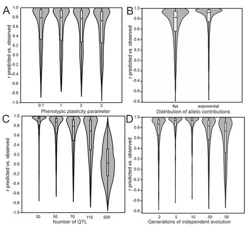
- Fig 4, what does it mean that r are negative? And for some panels (e.g. panel C, 500; panel E, 12),  basically 50% of the simulations show opposite signs. Please explain how shall we understand this, predictions cannot be trusted at all?

- line 494, yes, the trend is that the correlation is positive but it approximates zero pretty quickly. It will be important if the author explicitly tests for significance of such correlations and states what’s the actual limit in which he thinks the method is actually useful (e.g. less than 200 loci? Less than 20?). It is clear that the researcher doesn’t know a priori the genetic architecture of the trait, but this would make clear whether the proposed approach is truly useful for polygenic traits where hundreds or thousands of loci are expected to be involved.

- line 500. From Fig 1, while the trend again is consistent across distribution of effect sizes, it is clear than under the most realistic model (strong exponential), working with traits with more than 20 QTLs is not really a good idea under this model.

- the discussion uses a lot of imprecise statements that don’t make clear the actual limitations and potential for the method. For example, line 609 “ provided a sufficiently high number of populations is screened” how many?. Line 560 “increasing number of samples led to diminishing returns in statistical power beyond a certain threshold” which is such threshold? The discussion should be precise about the interpretation of the results and their implications for the implementation of this proposed approach in the field of complex traits in wild populations.

References

Futschik, A. and Schlötterer, C. 2010. The Next Generation of Molecular Markers From Massively Parallel Sequencing of Pooled DNA Samples. Genetics 186(1): 207-218. https://doi.org/10.1534/genetics.110.114397
Gienapp, P., Fior, S., Guillaume, F., Lasky, J. R., Sork, V. L. and Csilléry, K. 2017. Genomic Quantitative Genetics to Study Evolution in the Wild. Trends Ecol. Evol. 32(12): 897-908. https://doi.org/10.1016/j.tree.2017.09.004
Markus Pfenninger (2025) On the potential for GWAS with phenotypic population means and allele-frequency data (popGWAS). bioRxiv, ver.3 peer-reviewed and recommended by PCI Evol Biol https://doi.org/10.1101/2024.06.12.598621
Yeaman, S. and Whitlock, M. C. 2011. The genetic architecture of adaptation under migration-selection balance. Evolution 65(7): 1897-1911. https://doi.org/10.1111/j.1558-5646.2011.01269.x
The recommender in charge of the evaluation of the article and the reviewers declared that they have no conflict of interest (as defined in the code of conduct of PCI) with the authors or with the content of the article. The authors declared that they comply with the PCI rule of having no financial conflicts of interest in relation to the content of the article.
The author declares that he has received no specific funding for this study
Evaluation round #2
DOI or URL of the preprint: https://doi.org/10.1101/2024.06.12.598621
Version of the preprint: 2
Author's Reply, 12 Mar 2025
Decision by Frédéric Guillaume, posted 04 Mar 2025, validated 05 Mar 2025
Dear Markus,
Thank you for submitting your revised manuscript on popGWAS. The improvements are significant and I am willing to go on with recommendation pending some minor revisions. I attach a commented version of your manuscript where I have highlighted typos and places where corrections may be needed. I would also like to give you the opportunity to reply to the criticisms of reviewer 1. Many points raised by the reviewer are actually addressed in your discussion, I thus do not expect additional explanations for those points.
I would also like to ask you to clarify the iGWAS part as much as you can. Information on iGWAS in the supplementary material is missing and it would be informative for the readers to know more about the impact of population structure/relatedness on p-value inflation. I hope this would not require much more work from you.
I'd also recommend to avoid using "phenotypic plasticity" when referring to the "environmental variance" parameter. The two are used in the manuscript but it would be preferable to use only the environmental variance to refer to the random noise added to the genotypic value when computing the phenotype. A plastic response is expected to be more directional/predictive response to environmental variation rather than just noise.
Thank you for your contribution.
Best wishes,
Fred
Reviewed by Petri Kemppainen, 07 Feb 2025